Note

This page was generated from combosciplex.ipynb. Interactive online version: .

Predicting combinatorial drug perturbations#

In this tutorial, we train CPA on combo-sciplex dataset. This dataset is available here. See lotfollahi et al. for more info (also see how you can use external drug embedding to improve your prediction and predict unseen drugs). See Fig.3 in the paper for more analysis.

[1]:

import sys
#if branch is stable, will install via pypi, else will install from source
branch = "latest"
IN_COLAB = "google.colab" in sys.modules

if IN_COLAB and branch == "stable":
    !pip install cpa-tools
    !pip install scanpy
elif IN_COLAB and branch != "stable":
    !pip install --quiet --upgrade jsonschema
    !pip install git+https://github.com/theislab/cpa
    !pip install scanpy

[2]:

from sklearn.metrics import r2_score
import numpy as np

import os
# os.chdir('/home/mohsen/projects/cpa/')
# os.environ['CUDA_VISIBLE_DEVICES'] = '0'

[3]:

import cpa
import scanpy as sc

Global seed set to 0

[4]:

sc.settings.set_figure_params(dpi=100)

[5]:

data_path = '/home/mohsen/projects/cpa/datasets/combo_sciplex_prep_hvg_filtered.h5ad'

Data Loading#

[6]:

try:
    adata = sc.read(data_path)
except:
    import gdown
    gdown.download('https://drive.google.com/uc?export=download&id=1RRV0_qYKGTvD3oCklKfoZQFYqKJy4l6t')
    data_path = 'combo_sciplex_prep_hvg_filtered.h5ad'
    adata = sc.read(data_path)

adata

[6]:

AnnData object with n_obs × n_vars = 63378 × 5000
    obs: 'ncounts', 'well', 'plate', 'cell_line', 'replicate', 'time', 'dose_value', 'pathway1', 'pathway2', 'perturbation', 'target', 'pathway', 'dose_unit', 'celltype', 'disease', 'tissue_type', 'organism', 'perturbation_type', 'ngenes', 'percent_mito', 'percent_ribo', 'nperts', 'chembl-ID', 'condition', 'condition_ID', 'control', 'cell_type', 'smiles_rdkit', 'source', 'sample', 'Size_Factor', 'n.umi', 'RT_well', 'Drug1', 'Drug2', 'Well', 'n_genes', 'n_genes_by_counts', 'total_counts', 'total_counts_mt', 'pct_counts_mt', 'leiden', 'split', 'condition_old', 'pert_type', 'batch', 'split_1ct_MEC', 'split_2ct_MEC', 'split_3ct_MEC', 'batch_cov', 'batch_cov_cond', 'log_dose', 'cov_drug_dose'
    var: 'ensembl_id-0', 'ncounts-0', 'ncells-0', 'symbol-0', 'symbol-1', 'id-1', 'n_cells-1', 'mt-1', 'n_cells_by_counts-1', 'mean_counts-1', 'pct_dropout_by_counts-1', 'total_counts-1', 'highly_variable-1', 'means-1', 'dispersions-1', 'dispersions_norm-1', 'highly_variable', 'means', 'dispersions', 'dispersions_norm', 'highly_variable_nbatches', 'highly_variable_intersection'
    uns: 'cell_type_colors', 'hvg', 'neighbors', 'pathway1_colors', 'pca', 'rank_genes_groups_cov', 'rank_genes_groups_cov_detailed', 'source_colors', 'umap'
    obsm: 'X_pca', 'X_umap'
    varm: 'PCs'
    layers: 'counts'
    obsp: 'connectivities', 'distances'

Data setup#

IMPORTANT: Currenlty because of the standartized evaluation procedure, we need to provide adata.obs[‘control’] (0 if not control, 1 for cells to use as control). And we also need to provide de_genes in .uns[‘rank_genes_groups’].

In order to effectively assess the performance of the model, we have left out all cells perturbed by the following single/combinatorial perturbations. These cells are also used in the original paper for evaluation of CPA (See Figure 3 in the paper).

CHEMBL1213492+CHEMBL491473
CHEMBL483254+CHEMBL4297436
CHEMBL356066+CHEMBL402548
CHEMBL483254+CHEMBL383824
CHEMBL4297436+CHEMBL383824

[7]:

adata.obs['split_1ct_MEC'].value_counts()

[7]:

train    49683
ood       8209
valid     5486
Name: split_1ct_MEC, dtype: int64

[8]:

adata.X = adata.layers['counts'].copy()

[9]:

cpa.CPA.setup_anndata(adata,
                      perturbation_key='condition_ID',
                      dosage_key='log_dose',
                      control_group='CHEMBL504',
                      batch_key=None,
                      is_count_data=True,
                      categorical_covariate_keys=['cell_type'],
                      deg_uns_key='rank_genes_groups_cov',
                      deg_uns_cat_key='cov_drug_dose',
                      max_comb_len=2,
                     )

  0%|          | 0/63378 [00:00<?, ?it/s]

100%|██████████| 63378/63378 [00:01<00:00, 47875.85it/s]
100%|██████████| 63378/63378 [00:00<00:00, 562218.78it/s]
100%|██████████| 32/32 [00:00<00:00, 892.27it/s]
No GPU/TPU found, falling back to CPU. (Set TF_CPP_MIN_LOG_LEVEL=0 and rerun for more info.)

INFO     Generating sequential column names
INFO     Generating sequential column names
INFO     Generating sequential column names
INFO     Generating sequential column names

Training CPA#

You can specify all the parameters for the model in a dictionary of parameters. If they are not specified, default values will be selected.

ae_hparams are technical parameters of the architecture of the autoencoder.
- n_latent: number of latent dimensions for the autoencoder
- recon_loss: the type of reconstruction loss function to use
- doser_type: the type of doser to use
- n_hidden_encoder: number of hidden neurons in each hidden layer of the encoder
- n_layers_encoder: number of hidden layers in the encoder
- n_hidden_decoder: number of hidden neurons in each hidden layer of the decoder
- n_layers_decoder: number of hidden layers in the decoder
- use_batch_norm_encoder: if True, batch normalization will be used in the encoder
- use_layer_norm_encoder: if True, layer normalization will be used in the encoder
- use_batch_norm_decoder: if True, batch normalization will be used in the decoder
- use_layer_norm_decoder: if True, layer normalization will be used in the decoder
- dropout_rate_encoder: dropout rate used in the encoder
- dropout_rate_decoder: dropout rate used in the decoder
- variational: if True, variational autoencoder will be employed as the main perturbation response predictor
- seed: number for setting the seed for generating random numbers.
trainer_params are training parameters of CPA.
- n_epochs_adv_warmup: number of epochs for adversarial warmup
- n_epochs_kl_warmup: number of epochs for KL divergence warmup
- n_epochs_pretrain_ae: number of epochs to pre-train the autoencoder
- adv_steps: number of steps used to train adversarial classifiers after a single step of training the autoencoder
- mixup_alpha: mixup interpolation coefficient
- n_epochs_mixup_warmup: number of epochs for mixup warmup
- lr: learning rate of the trainer
- wd: weight decay of the trainer
- doser_lr: learning rate of doser parameters
- doser_wd: weight decay of doser parameters
- adv_lr: learning rate of adversarial classifiers
- adv_wd: weight decay rate of adversarial classifiers
- pen_adv: penalty for adversarial classifiers
- reg_adv: regularization for adversarial classifiers
- n_layers_adv: number of hidden layers in adversarial classifiers
- n_hidden_adv: number of hidden neurons in each hidden layer of adversarial classifiers
- use_batch_norm_adv: if True, batch normalization will be used in the adversarial classifiers
- use_layer_norm_adv: if True, layer normalization will be used in the adversarial classifiers
- dropout_rate_adv: dropout rate used in the adversarial classifiers
- step_size_lr: learning rate step size
- do_clip_grad: if True, gradient clipping will be used
- adv_loss: the type of loss function to use for adversarial training
- gradient_clip_value: value to clip gradients to, if do_clip_grad is True

[9]:

ae_hparams = {
    "n_latent": 128,
    "recon_loss": "nb",
    "doser_type": "logsigm",
    "n_hidden_encoder": 512,
    "n_layers_encoder": 3,
    "n_hidden_decoder": 512,
    "n_layers_decoder": 3,
    "use_batch_norm_encoder": True,
    "use_layer_norm_encoder": False,
    "use_batch_norm_decoder": True,
    "use_layer_norm_decoder": False,
    "dropout_rate_encoder": 0.1,
    "dropout_rate_decoder": 0.1,
    "variational": False,
    "seed": 434,
}

trainer_params = {
    "n_epochs_kl_warmup": None,
    "n_epochs_pretrain_ae": 30,
    "n_epochs_adv_warmup": 50,
    "n_epochs_mixup_warmup": 3,
    "mixup_alpha": 0.1,
    "adv_steps": 2,
    "n_hidden_adv": 64,
    "n_layers_adv": 2,
    "use_batch_norm_adv": True,
    "use_layer_norm_adv": False,
    "dropout_rate_adv": 0.3,
    "reg_adv": 20.0,
    "pen_adv": 20.0,
    "lr": 0.0003,
    "wd": 4e-07,
    "adv_lr": 0.0003,
    "adv_wd": 4e-07,
    "adv_loss": "cce",
    "doser_lr": 0.0003,
    "doser_wd": 4e-07,
    "do_clip_grad": False,
    "gradient_clip_value": 1.0,
    "step_size_lr": 45,
}

Model instantiation#

NOTE: Run the following 3 cells if you haven’t already trained CPA from scratch.

Here, we create a CPA model using cpa.CPA given all hyper-parameters.

[10]:

adata.obs['split_1ct_MEC'].value_counts()

[10]:

train    49683
ood       8209
valid     5486
Name: split_1ct_MEC, dtype: int64

[11]:

model = cpa.CPA(adata=adata,
                split_key='split_1ct_MEC',
                train_split='train',
                valid_split='valid',
                test_split='ood',
                **ae_hparams,
               )

Global seed set to 434

Training CPA#

After creating a CPA object, we train the model with the following arguments: * max_epochs: Maximum number of epochs to train the models. * use_gpu: If True, will use the available GPU to train the model. * batch_size: Number of samples to use in each mini-batches. * early_stopping_patience: Number of epochs with no improvement in early stopping callback. * check_val_every_n_epoch: Interval of checking validation losses. * save_path: Path to save the model after the training has finished.

[12]:

model.train(max_epochs=2000,
            use_gpu=True,
            batch_size=128,
            plan_kwargs=trainer_params,
            early_stopping_patience=10,
            check_val_every_n_epoch=5,
            save_path='/home/mohsen/projects/cpa/lightning_logs/combo/',
           )

100%|██████████| 32/32 [00:00<00:00, 69.28it/s]
GPU available: True (cuda), used: True
TPU available: False, using: 0 TPU cores
IPU available: False, using: 0 IPUs
HPU available: False, using: 0 HPUs
You are using a CUDA device ('NVIDIA RTX A6000') that has Tensor Cores. To properly utilize them, you should set `torch.set_float32_matmul_precision('medium' | 'high')` which will trade-off precision for performance. For more details, read https://pytorch.org/docs/stable/generated/torch.set_float32_matmul_precision.html#torch.set_float32_matmul_precision
LOCAL_RANK: 0 - CUDA_VISIBLE_DEVICES: [0]

Epoch 5/2000:   0%|          | 4/2000 [01:06<9:13:26, 16.64s/it, v_num=1, recon=1.3e+3, r2_mean=0.81, adv_loss=2.09, acc_pert=0.204]


Epoch 00004: cpa_metric reached. Module best state updated.

Epoch 10/2000:   0%|          | 9/2000 [02:31<9:19:32, 16.86s/it, v_num=1, recon=1.27e+3, r2_mean=0.826, adv_loss=1.9, acc_pert=0.254, val_recon=1.29e+3, disnt_basal=0.0684, disnt_after=0.101, val_r2_mean=0.816, val_KL=nan]


Epoch 00009: cpa_metric reached. Module best state updated.


disnt_basal = 0.05681036256785612
disnt_after = 0.09083146896966879
val_r2_mean = 0.8232210043019584
val_r2_var = 0.4547786588474683
Epoch 15/2000:   1%|          | 14/2000 [03:53<9:05:00, 16.47s/it, v_num=1, recon=1.26e+3, r2_mean=0.831, adv_loss=1.87, acc_pert=0.27, val_recon=1.27e+3, disnt_basal=0.0568, disnt_after=0.0908, val_r2_mean=0.823, val_KL=nan]


Epoch 00014: cpa_metric reached. Module best state updated.

Epoch 20/2000:   1%|          | 19/2000 [05:14<8:51:41, 16.10s/it, v_num=1, recon=1.25e+3, r2_mean=0.834, adv_loss=1.87, acc_pert=0.272, val_recon=1.26e+3, disnt_basal=0.0528, disnt_after=0.0864, val_r2_mean=0.826, val_KL=nan]


Epoch 00019: cpa_metric reached. Module best state updated.


disnt_basal = 0.04882907598151999
disnt_after = 0.08111213412189941
val_r2_mean = 0.8247866788097772
val_r2_var = 0.46757752377354017
Epoch 25/2000:   1%|          | 24/2000 [06:39<9:06:15, 16.59s/it, v_num=1, recon=1.24e+3, r2_mean=0.836, adv_loss=1.89, acc_pert=0.271, val_recon=1.25e+3, disnt_basal=0.0488, disnt_after=0.0811, val_r2_mean=0.825, val_KL=nan]


Epoch 00024: cpa_metric reached. Module best state updated.

Epoch 30/2000:   1%|▏         | 29/2000 [08:03<9:14:04, 16.87s/it, v_num=1, recon=1.24e+3, r2_mean=0.836, adv_loss=1.9, acc_pert=0.274, val_recon=1.25e+3, disnt_basal=0.0457, disnt_after=0.0792, val_r2_mean=0.831, val_KL=nan]
disnt_basal = 0.04493595321002729
disnt_after = 0.07789831388664292
val_r2_mean = 0.8299014887505352
val_r2_var = 0.45619733785284466
Epoch 40/2000:   2%|▏         | 39/2000 [10:36<8:03:53, 14.81s/it, v_num=1, recon=1.23e+3, r2_mean=0.837, adv_loss=3.13, acc_pert=0.1, val_recon=1.25e+3, disnt_basal=0.0368, disnt_after=0.0695, val_r2_mean=0.829, val_KL=nan]
disnt_basal = 0.03420521420534983
disnt_after = 0.06885151633917305
val_r2_mean = 0.8300215740873791
val_r2_var = 0.4536893434363568
Epoch 45/2000:   2%|▏         | 44/2000 [11:57<8:30:35, 15.66s/it, v_num=1, recon=1.23e+3, r2_mean=0.838, adv_loss=3.23, acc_pert=0.0721, val_recon=1.25e+3, disnt_basal=0.0342, disnt_after=0.0689, val_r2_mean=0.83, val_KL=nan]


Epoch 00044: cpa_metric reached. Module best state updated.

Epoch 50/2000:   2%|▏         | 49/2000 [13:13<8:06:09, 14.95s/it, v_num=1, recon=1.23e+3, r2_mean=0.837, adv_loss=3.23, acc_pert=0.0647, val_recon=1.25e+3, disnt_basal=0.0334, disnt_after=0.0698, val_r2_mean=0.83, val_KL=nan]
disnt_basal = 0.033261220440177576
disnt_after = 0.06962234036567172
val_r2_mean = 0.8230554203589677
val_r2_var = 0.4512327983674288
Epoch 60/2000:   3%|▎         | 59/2000 [15:52<8:34:28, 15.90s/it, v_num=1, recon=1.23e+3, r2_mean=0.836, adv_loss=3.25, acc_pert=0.0561, val_recon=1.25e+3, disnt_basal=0.0327, disnt_after=0.0699, val_r2_mean=0.823, val_KL=nan]
disnt_basal = 0.03283145492859847
disnt_after = 0.07138437578504499
val_r2_mean = 0.8216465924869693
val_r2_var = 0.4576330099764238
Epoch 70/2000:   3%|▎         | 69/2000 [18:22<7:49:42, 14.59s/it, v_num=1, recon=1.22e+3, r2_mean=0.837, adv_loss=3.26, acc_pert=0.0511, val_recon=1.26e+3, disnt_basal=0.0328, disnt_after=0.0715, val_r2_mean=0.823, val_KL=nan]
disnt_basal = 0.03221930997610452
disnt_after = 0.07143286619959249
val_r2_mean = 0.8243548340085156
val_r2_var = 0.4545298452111304
Epoch 80/2000:   4%|▍         | 79/2000 [20:56<8:16:32, 15.51s/it, v_num=1, recon=1.22e+3, r2_mean=0.839, adv_loss=3.27, acc_pert=0.0484, val_recon=1.26e+3, disnt_basal=0.032, disnt_after=0.0723, val_r2_mean=0.815, val_KL=nan]
disnt_basal = 0.0320174356914021
disnt_after = 0.07160127920616723
val_r2_mean = 0.8239223117915013
val_r2_var = 0.4527030767477002
Epoch 90/2000:   4%|▍         | 89/2000 [23:34<8:11:34, 15.43s/it, v_num=1, recon=1.22e+3, r2_mean=0.839, adv_loss=3.27, acc_pert=0.0465, val_recon=1.26e+3, disnt_basal=0.0321, disnt_after=0.0726, val_r2_mean=0.82, val_KL=nan]
disnt_basal = 0.03193920512355714
disnt_after = 0.07343884982388675
val_r2_mean = 0.8206448153586611
val_r2_var = 0.44997947452614184
Epoch 95/2000:   5%|▍         | 95/2000 [25:05<8:23:09, 15.85s/it, v_num=1, recon=1.22e+3, r2_mean=0.838, adv_loss=3.27, acc_pert=0.0471, val_recon=1.26e+3, disnt_basal=0.0323, disnt_after=0.0727, val_r2_mean=0.823, val_KL=nan]

[13]:

cpa.pl.plot_history(model)

../_images/tutorials_combosciplex_25_0.png

If you already trained CPA, you can restore model weights by running the following cell:

[9]:

model = cpa.CPA.load(dir_path='/home/mohsen/projects/cpa/lightning_logs/combo/',
                     adata=adata, use_gpu=True)

INFO     File /home/mohsen/projects/cpa/lightning_logs/combo/model.pt already downloaded

100%|██████████| 63378/63378 [00:00<00:00, 63731.38it/s]
100%|██████████| 63378/63378 [00:00<00:00, 687996.21it/s]
100%|██████████| 32/32 [00:00<00:00, 1221.06it/s]
No GPU/TPU found, falling back to CPU. (Set TF_CPP_MIN_LOG_LEVEL=0 and rerun for more info.)
Global seed set to 434

Latent space UMAP visualization#

Here, we visualize the latent representations of all cells. We computed basal and final latent representations with model.get_latent_representation function.

[10]:

latent_outputs = model.get_latent_representation(adata, batch_size=1024)

100%|██████████| 62/62 [00:03<00:00, 16.44it/s]

[13]:

sc.settings.verbosity = 3

[11]:

latent_basal_adata = latent_outputs['latent_basal']
latent_adata = latent_outputs['latent_after']

[12]:

sc.pp.neighbors(latent_basal_adata)
sc.tl.umap(latent_basal_adata)

WARNING: You’re trying to run this on 128 dimensions of `.X`, if you really want this, set `use_rep='X'`.
         Falling back to preprocessing with `sc.pp.pca` and default params.

[13]:

latent_basal_adata

[13]:

AnnData object with n_obs × n_vars = 63378 × 128
    obs: 'ncounts', 'well', 'plate', 'cell_line', 'replicate', 'time', 'dose_value', 'pathway1', 'pathway2', 'perturbation', 'target', 'pathway', 'dose_unit', 'celltype', 'disease', 'tissue_type', 'organism', 'perturbation_type', 'ngenes', 'percent_mito', 'percent_ribo', 'nperts', 'chembl-ID', 'condition', 'condition_ID', 'control', 'cell_type', 'smiles_rdkit', 'source', 'sample', 'Size_Factor', 'n.umi', 'RT_well', 'Drug1', 'Drug2', 'Well', 'n_genes', 'n_genes_by_counts', 'total_counts', 'total_counts_mt', 'pct_counts_mt', 'leiden', 'split', 'condition_old', 'pert_type', 'batch', 'split_1ct_MEC', 'split_2ct_MEC', 'split_3ct_MEC', 'batch_cov', 'batch_cov_cond', 'log_dose', 'cov_drug_dose', 'CPA_cat', 'CPA_CHEMBL504', '_scvi_condition_ID', '_scvi_cell_type', '_scvi_CPA_cat'
    uns: 'neighbors', 'umap'
    obsm: 'X_pca', 'X_umap'
    obsp: 'distances', 'connectivities'

The basal representation should be free of the variation(s) of the `’condition_ID’ as observed below

[14]:

sc.pl.umap(latent_basal_adata, color=['condition_ID'], frameon=False, wspace=0.2)

../_images/tutorials_combosciplex_36_0.png

Here, you can visualize that when the drug embedding is added to the basal representation, the cells treated with different drugs will be separated.

[15]:

sc.pp.neighbors(latent_adata)
sc.tl.umap(latent_adata)

WARNING: You’re trying to run this on 128 dimensions of `.X`, if you really want this, set `use_rep='X'`.
         Falling back to preprocessing with `sc.pp.pca` and default params.

[16]:

sc.pl.umap(latent_adata, color=['condition_ID'], frameon=False, wspace=0.2)

../_images/tutorials_combosciplex_39_0.png

Evaluation#

Next, we will evaluate the model’s prediction performance on the whole dataset, including OOD (test) cells. The model will report metrics on how well we have captured the variation in top n differentially expressed genes when compared to control cells (DMSO, CHEMBL 504) for each condition. The metrics calculate the mean accuracy (r2_mean_deg), the variance (r2_var_deg) and similar metrics (r2_mean_lfc_deg and log fold change)to measure the log fold change of the predicted cells vs control((LFC(control, ground truth) ~ LFC(control, predicted cells)). The R2 is the sklearn.metrics.r2_score from sklearn.

[20]:

model.predict(adata, batch_size=1024)

100%|██████████| 62/62 [00:08<00:00,  7.55it/s]

[21]:

import numpy as np
import pandas as pd
from sklearn.metrics import r2_score
from collections import defaultdict
from tqdm import tqdm

n_top_degs = [10, 20, 50, None] # None means all genes

results = defaultdict(list)
ctrl_adata = adata[adata.obs['condition_ID'] == 'CHEMBL504'].copy()
for cat in tqdm(adata.obs['cov_drug_dose'].unique()):
    if 'CHEMBL504' not in cat:
        cat_adata = adata[adata.obs['cov_drug_dose'] == cat].copy()

        deg_cat = f'{cat}'
        deg_list = adata.uns['rank_genes_groups_cov'][deg_cat]

        x_true = cat_adata.layers['counts'].toarray()
        x_pred = cat_adata.obsm['CPA_pred']
        x_ctrl = ctrl_adata.layers['counts'].toarray()

        x_true = np.log1p(x_true)
        x_pred = np.log1p(x_pred)
        x_ctrl = np.log1p(x_ctrl)

        for n_top_deg in n_top_degs:
            if n_top_deg is not None:
                degs = np.where(np.isin(adata.var_names, deg_list[:n_top_deg]))[0]
            else:
                degs = np.arange(adata.n_vars)
                n_top_deg = 'all'

            x_true_deg = x_true[:, degs]
            x_pred_deg = x_pred[:, degs]
            x_ctrl_deg = x_ctrl[:, degs]

            r2_mean_deg = r2_score(x_true_deg.mean(0), x_pred_deg.mean(0))
            r2_var_deg = r2_score(x_true_deg.var(0), x_pred_deg.var(0))

            r2_mean_lfc_deg = r2_score(x_true_deg.mean(0) - x_ctrl_deg.mean(0), x_pred_deg.mean(0) - x_ctrl_deg.mean(0))
            r2_var_lfc_deg = r2_score(x_true_deg.var(0) - x_ctrl_deg.var(0), x_pred_deg.var(0) - x_ctrl_deg.var(0))

            cov, cond, dose = cat.split('_')

            results['cell_type'].append(cov)
            results['condition'].append(cond)
            results['dose'].append(dose)
            results['n_top_deg'].append(n_top_deg)
            results['r2_mean_deg'].append(r2_mean_deg)
            results['r2_var_deg'].append(r2_var_deg)
            results['r2_mean_lfc_deg'].append(r2_mean_lfc_deg)
            results['r2_var_lfc_deg'].append(r2_var_lfc_deg)

df = pd.DataFrame(results)

100%|██████████| 32/32 [00:15<00:00,  2.10it/s]

[22]:

df[df['n_top_deg'] == 20]

[22]:

	cell_type	condition	dose	n_top_deg	r2_mean_deg	r2_var_deg	r2_mean_lfc_deg	r2_var_lfc_deg
1	A549	CHEMBL483254	3.0	20	0.967421	0.379410	0.991763	0.807461
5	A549	CHEMBL491473+CHEMBL2170177	3.0+3.0	20	0.962717	-0.623639	0.475555	-18.077933
9	A549	CHEMBL1213492+CHEMBL257991	3.0+3.0	20	0.869307	-2.036985	0.509137	-4.899390
13	A549	CHEMBL483254+46245047	3.0+3.0	20	0.970208	0.456921	0.991650	0.813883
17	A549	CHEMBL483254+CHEMBL2170177	3.0+3.0	20	0.968506	0.261224	0.990237	0.713178
21	A549	CHEMBL356066	3.0	20	0.935541	0.174922	0.978043	0.749956
25	A549	CHEMBL356066+CHEMBL2170177	3.0+3.0	20	0.947310	0.335508	0.983684	0.805031
29	A549	CHEMBL483254+CHEMBL1200485	3.0+3.0	20	0.969701	0.390255	0.990890	0.765023
33	A549	CHEMBL1213492+CHEMBL491473	3.0+3.0	20	0.641915	-1.228658	0.514041	-3.090287
37	A549	CHEMBL1213492	3.0	20	0.895580	-2.776267	0.699633	-1.395146
41	A549	CHEMBL356066+CHEMBL402548	3.0+3.0	20	0.852191	-0.223018	0.954963	0.675036
45	A549	CHEMBL483254+CHEMBL1421	3.0+3.0	20	0.957488	0.265722	0.988489	0.744195
49	A549	CHEMBL1213492+CHEMBL109480	3.0+3.0	20	0.818061	-0.812865	0.921359	-1.243313
53	A549	CHEMBL1213492+CHEMBL460499	3.0+3.0	20	0.899389	-2.703637	0.767022	-3.808961
57	A549	CHEMBL483254+CHEMBL4297436	3.0+3.0	20	0.919735	0.375467	0.976873	0.779405
61	A549	CHEMBL483254+CHEMBL257991	3.0+3.0	20	0.956477	0.274221	0.987838	0.750310
65	A549	CHEMBL483254+CHEMBL601719	3.0+3.0	20	0.964190	0.293376	0.988411	0.725715
69	A549	CHEMBL383824+CHEMBL2354444	3.0+3.0	20	0.956984	-0.765112	0.971313	0.258857
73	A549	CHEMBL1213492+CHEMBL4297436	3.0+3.0	20	0.895441	-0.618630	0.691770	-0.443078
77	A549	CHEMBL1213492+CHEMBL1200485	3.0+3.0	20	0.941326	0.245628	0.971003	0.768830
81	A549	CHEMBL483254+CHEMBL383824	3.0+3.0	20	0.756303	-0.656045	0.920463	0.393564
85	A549	CHEMBL383824	3.0	20	0.908421	-1.523500	0.874507	-0.707571
89	A549	CHEMBL483254+CHEMBL116438	3.0+3.0	20	0.971904	0.506375	0.992483	0.840598
93	A549	CHEMBL1213492+CHEMBL1421	3.0+3.0	20	0.902487	-2.819458	0.864271	-2.265155
97	A549	CHEMBL4297436+CHEMBL383824	3.0+3.0	20	0.740274	-0.753398	0.830227	0.074761
101	A549	CHEMBL356066+CHEMBL1421	3.0+3.0	20	0.929562	0.274883	0.982519	0.785440
105	A549	CHEMBL4297436	3.0	20	0.796419	-3.606721	-0.526552	-14.992378
109	A549	CHEMBL1213492+CHEMBL116438	3.0+3.0	20	0.919315	-2.284597	0.721021	-4.020803
113	A549	CHEMBL1213492+CHEMBL601719	3.0+3.0	20	0.839387	-0.597107	0.807445	-2.828869
117	A549	46245047+CHEMBL491473	3.0+3.0	20	0.883893	-2.641516	-1.024542	-25.130354
121	A549	CHEMBL1421	3.0	20	0.950044	-0.274987	0.887869	-1.288966

n_top_deg shows how many DEGs genes were used to calculate the metric.

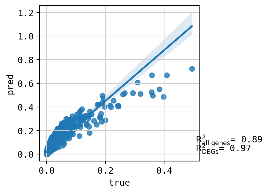
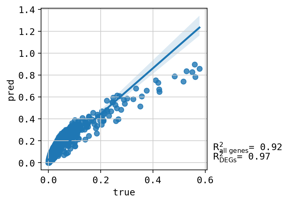
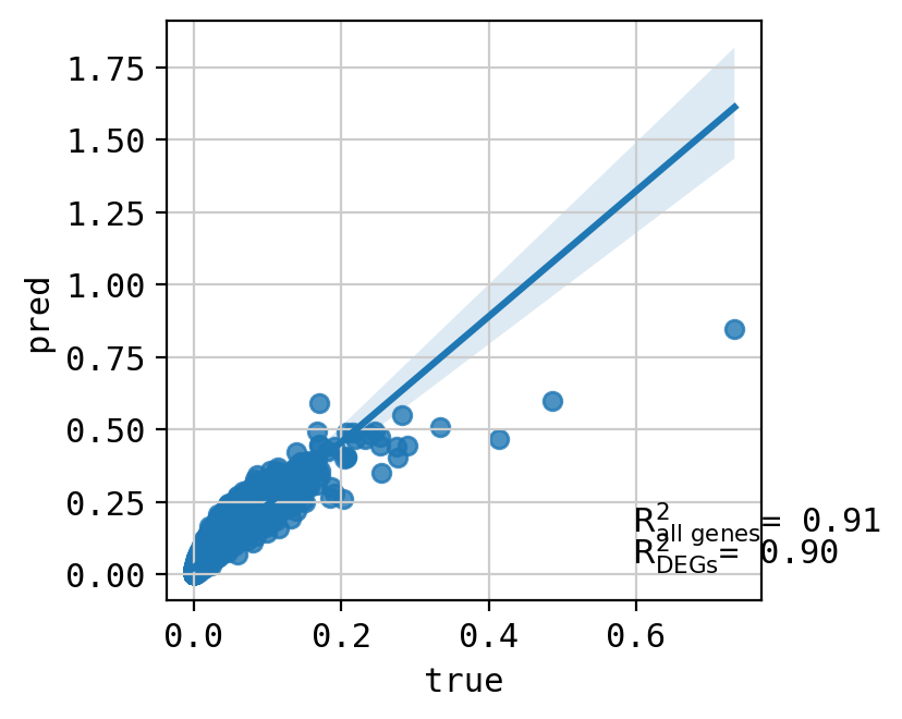
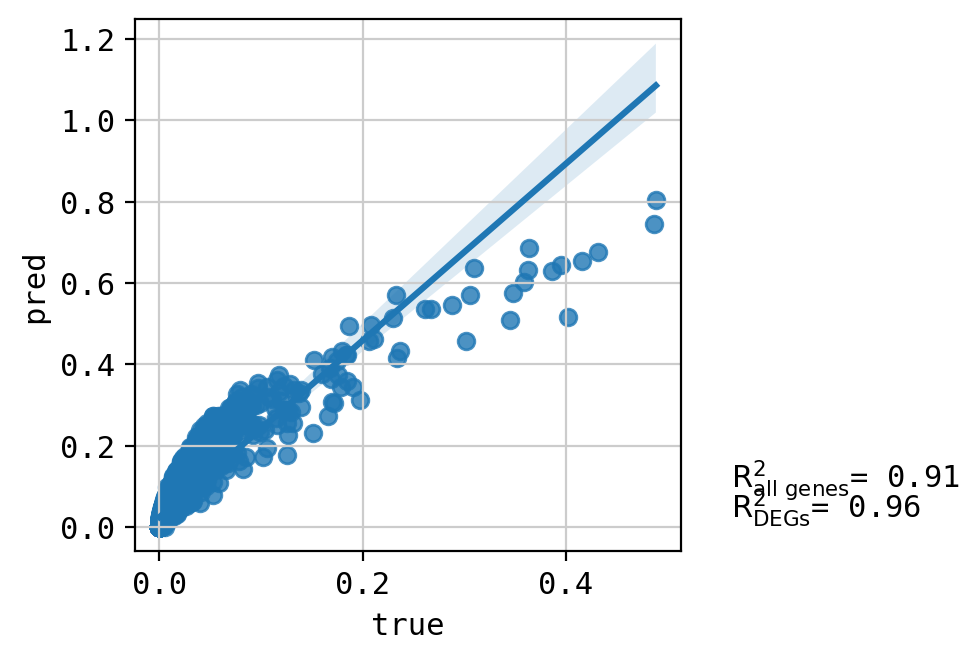
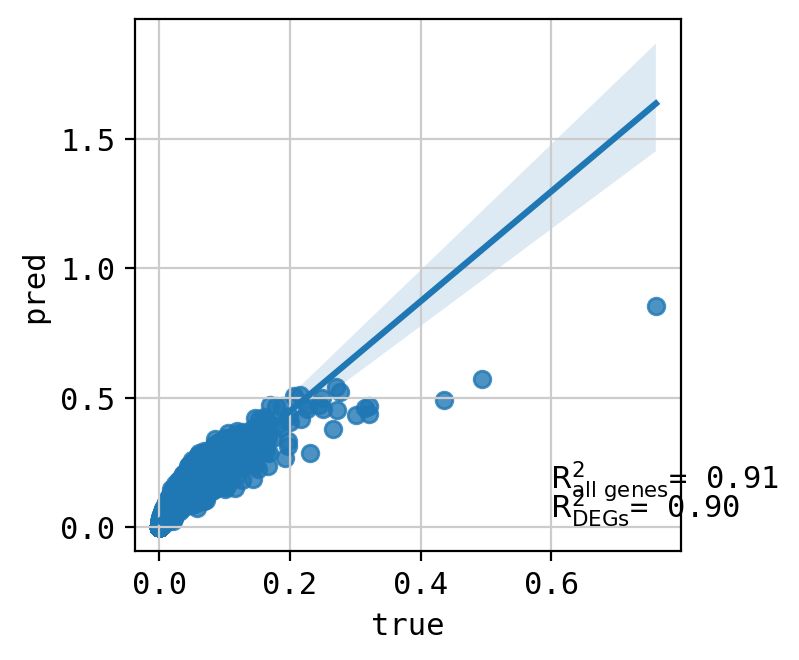
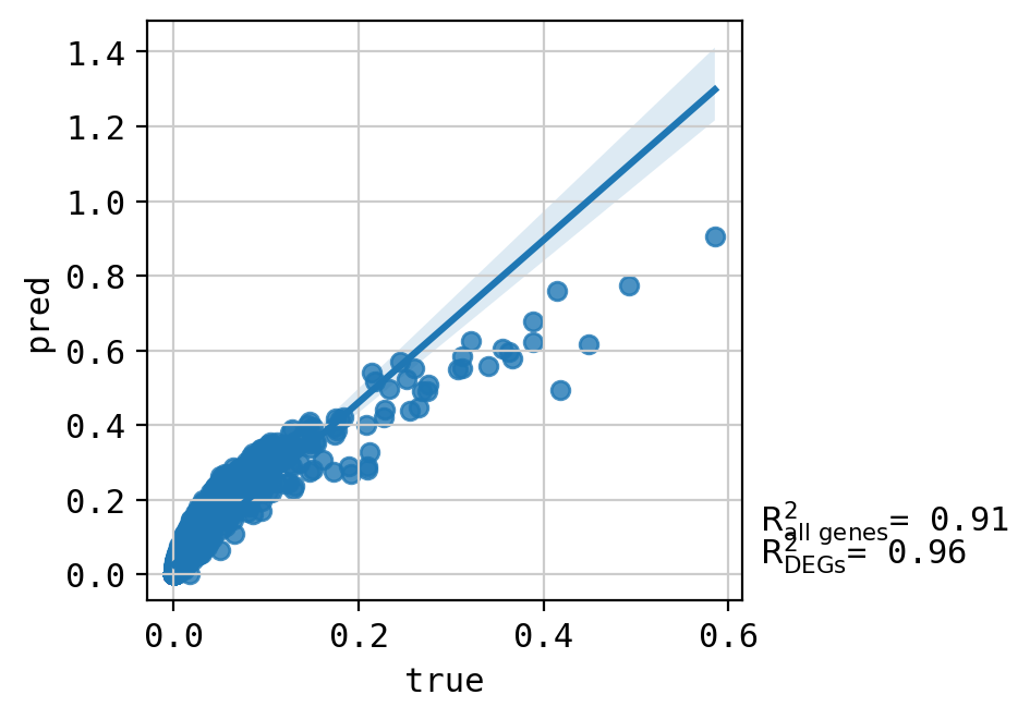
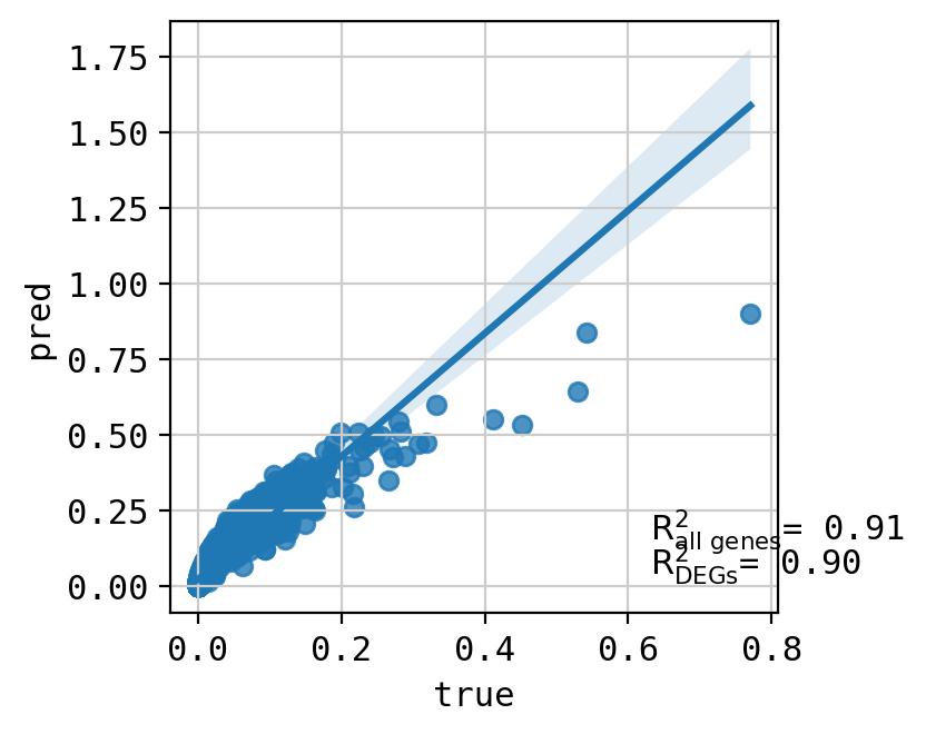
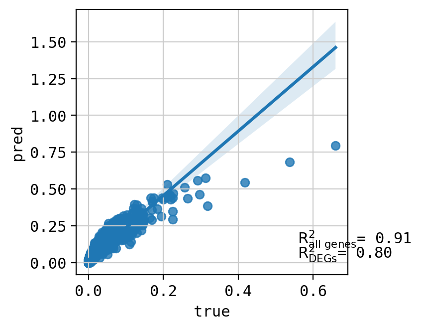
We can further visualize these per condition

[21]:

for cat in adata.obs["cov_drug_dose"].unique():
    if "CHEMBL504" not in cat:
        cat_adata = adata[adata.obs["cov_drug_dose"] == cat].copy()

        cat_adata.X = np.log1p(cat_adata.layers["counts"].A)
        cat_adata.obsm["CPA_pred"] = np.log1p(cat_adata.obsm["CPA_pred"])

        deg_list = adata.uns["rank_genes_groups_cov"][f'{cat}'][:20]

        print(cat, f"{cat_adata.shape}")
        cpa.pl.mean_plot(
            cat_adata,
            pred_obsm_key="CPA_pred",
            path_to_save=None,
            deg_list=deg_list,
            # gene_list=deg_list[:5],
            show=True,
            verbose=True,
        )

A549_CHEMBL483254_3.0 (1578, 5000)
Top 20 DEGs var:  0.9674240647799511
All genes var:  0.30564831092038325

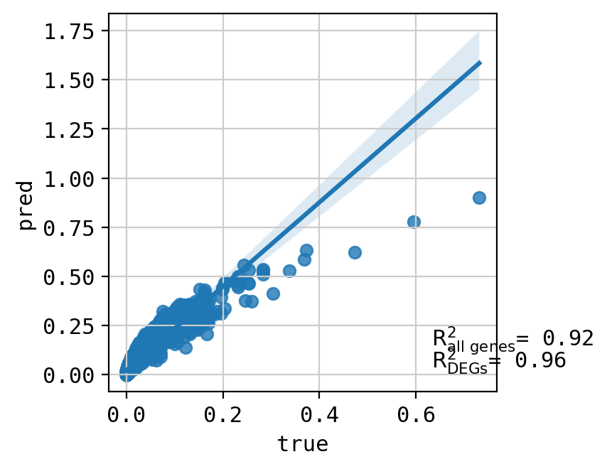
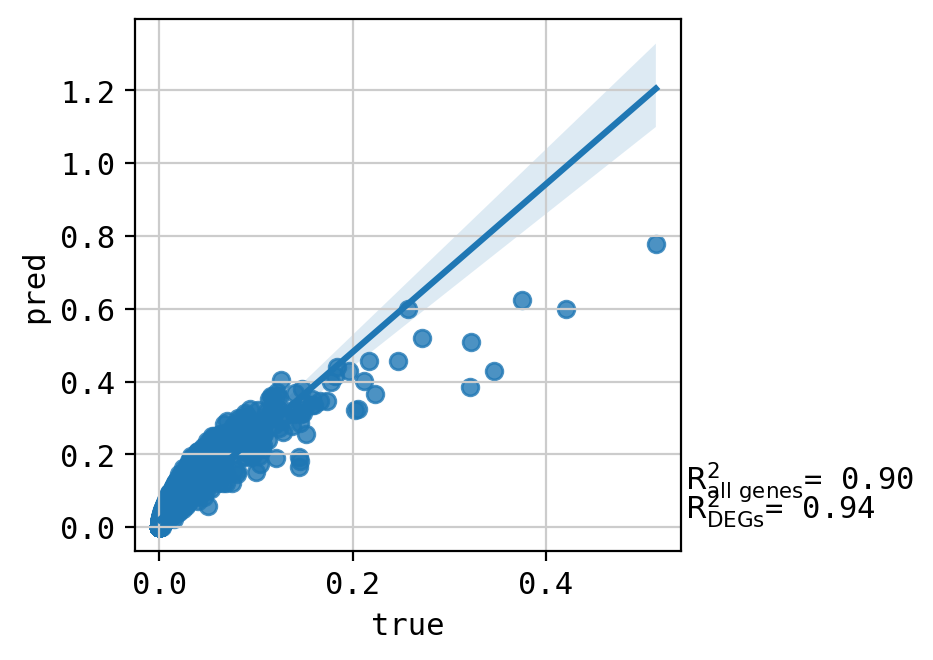
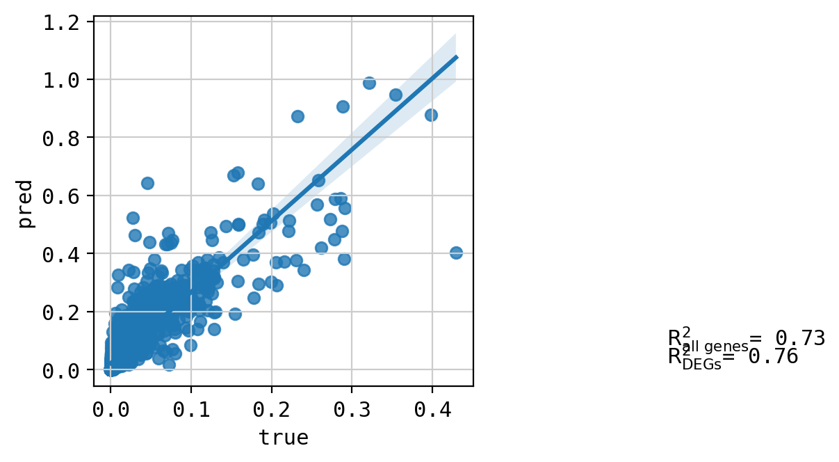
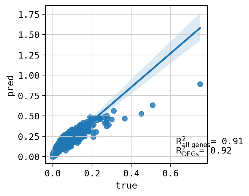
../_images/tutorials_combosciplex_47_1.png

A549_CHEMBL491473+CHEMBL2170177_3.0+3.0 (2161, 5000)
Top 20 DEGs var:  0.9627187921391631
All genes var:  0.3677191966657336

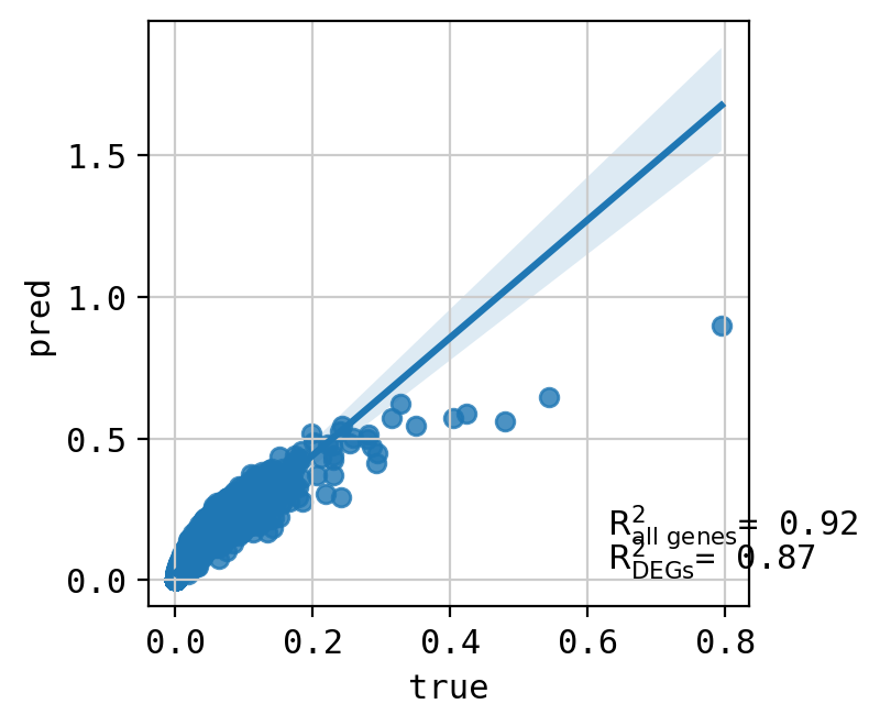
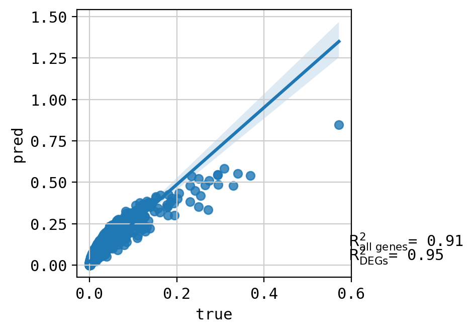
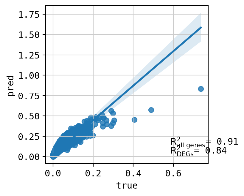
../_images/tutorials_combosciplex_47_3.png

A549_CHEMBL1213492+CHEMBL257991_3.0+3.0 (2260, 5000)
Top 20 DEGs var:  0.8693143108409295
All genes var:  0.32830499840643523

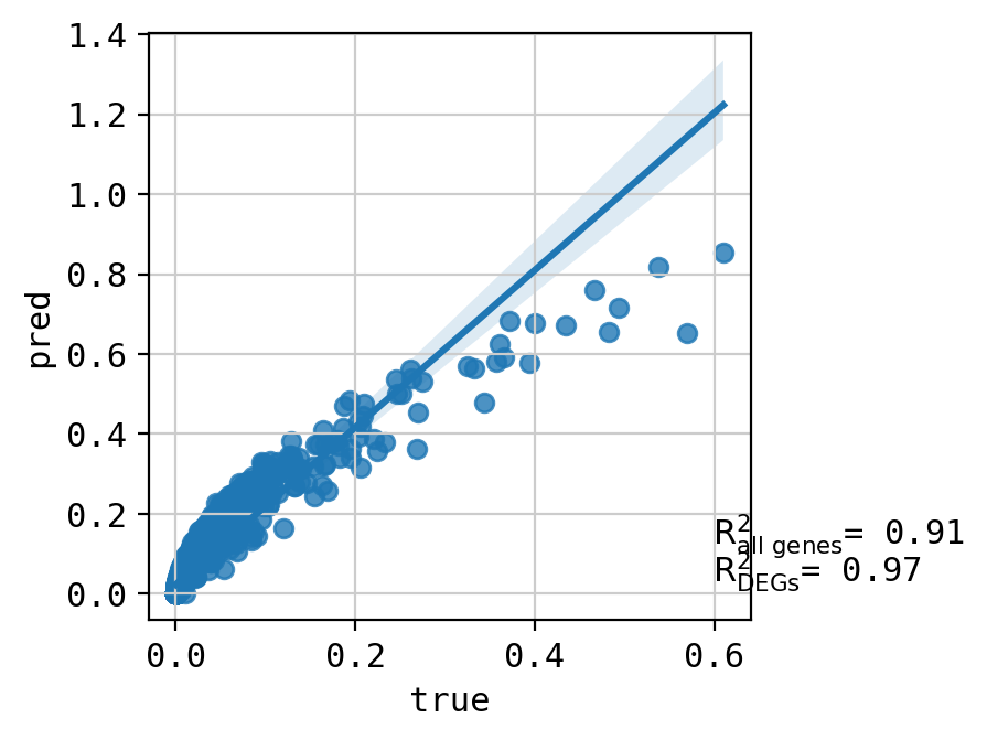
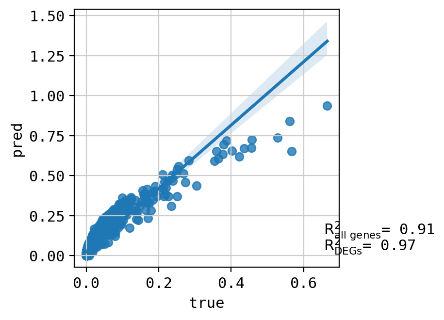
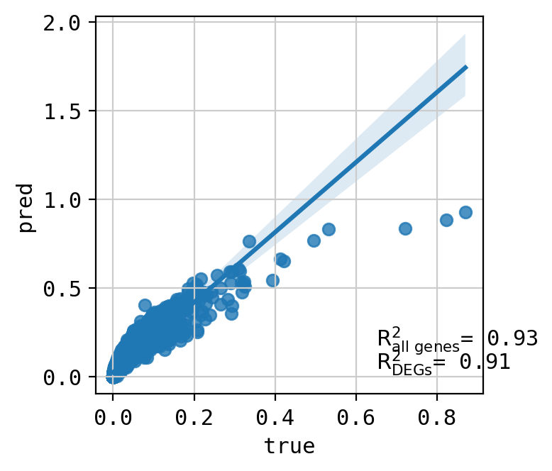
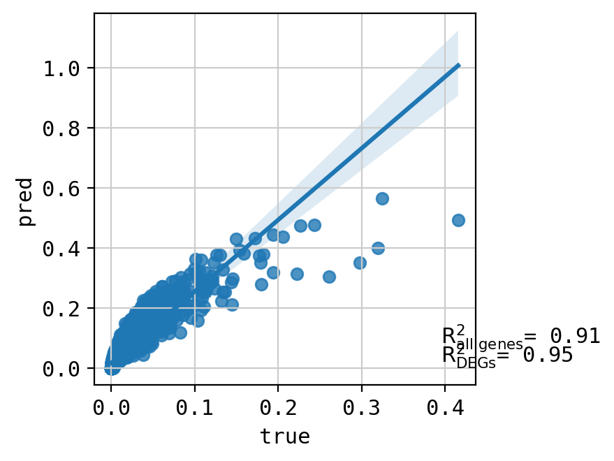
../_images/tutorials_combosciplex_47_5.png

A549_CHEMBL483254+46245047_3.0+3.0 (1889, 5000)
Top 20 DEGs var:  0.970209673172722
All genes var:  0.42205899370560873

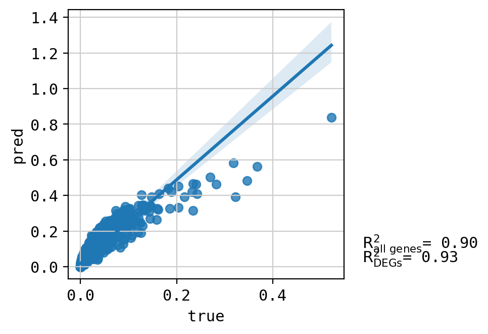
../_images/tutorials_combosciplex_47_7.png

A549_CHEMBL483254+CHEMBL2170177_3.0+3.0 (1814, 5000)
Top 20 DEGs var:  0.968507309155123
All genes var:  0.34981293176885053

../_images/tutorials_combosciplex_47_9.png

A549_CHEMBL356066_3.0 (1869, 5000)
Top 20 DEGs var:  0.9355440682391789
All genes var:  0.2884194789856178

../_images/tutorials_combosciplex_47_11.png

A549_CHEMBL356066+CHEMBL2170177_3.0+3.0 (3298, 5000)
Top 20 DEGs var:  0.947310703191107
All genes var:  0.29835334467419505

../_images/tutorials_combosciplex_47_13.png

A549_CHEMBL483254+CHEMBL1200485_3.0+3.0 (2013, 5000)
Top 20 DEGs var:  0.969701753626122
All genes var:  0.3981900429521762

../_images/tutorials_combosciplex_47_15.png

A549_CHEMBL1213492+CHEMBL491473_3.0+3.0 (2783, 5000)
Top 20 DEGs var:  0.6419152626745332
All genes var:  0.2886166540493904

../_images/tutorials_combosciplex_47_17.png

A549_CHEMBL1213492_3.0 (1682, 5000)
Top 20 DEGs var:  0.895586478486223
All genes var:  0.297598943550916

../_images/tutorials_combosciplex_47_19.png

A549_CHEMBL356066+CHEMBL402548_3.0+3.0 (1939, 5000)
Top 20 DEGs var:  0.8521916098477549
All genes var:  0.17711482339864315

../_images/tutorials_combosciplex_47_21.png

A549_CHEMBL483254+CHEMBL1421_3.0+3.0 (1955, 5000)
Top 20 DEGs var:  0.9574904467120635
All genes var:  0.306132009112956

../_images/tutorials_combosciplex_47_23.png

A549_CHEMBL1213492+CHEMBL109480_3.0+3.0 (1310, 5000)
Top 20 DEGs var:  0.8180723568291253
All genes var:  0.3774129061389593

../_images/tutorials_combosciplex_47_25.png

A549_CHEMBL1213492+CHEMBL460499_3.0+3.0 (2692, 5000)
Top 20 DEGs var:  0.8993912250910164
All genes var:  0.2901722828562925

../_images/tutorials_combosciplex_47_27.png

A549_CHEMBL483254+CHEMBL4297436_3.0+3.0 (1971, 5000)
Top 20 DEGs var:  0.9197375227935931
All genes var:  0.296415384031939

../_images/tutorials_combosciplex_47_29.png

A549_CHEMBL483254+CHEMBL257991_3.0+3.0 (1826, 5000)
Top 20 DEGs var:  0.9564792218882475
All genes var:  0.3108349920170532

../_images/tutorials_combosciplex_47_31.png

A549_CHEMBL483254+CHEMBL601719_3.0+3.0 (1641, 5000)
Top 20 DEGs var:  0.9641929190351832
All genes var:  0.355529304962353

../_images/tutorials_combosciplex_47_33.png

A549_CHEMBL383824+CHEMBL2354444_3.0+3.0 (476, 5000)
Top 20 DEGs var:  0.9569839749219734
All genes var:  0.392374583026051

../_images/tutorials_combosciplex_47_35.png

A549_CHEMBL1213492+CHEMBL4297436_3.0+3.0 (2353, 5000)
Top 20 DEGs var:  0.8954470865997979
All genes var:  0.3615505179215007

../_images/tutorials_combosciplex_47_37.png

A549_CHEMBL1213492+CHEMBL1200485_3.0+3.0 (2734, 5000)
Top 20 DEGs var:  0.9413281346007902
All genes var:  0.23785497259112265

../_images/tutorials_combosciplex_47_39.png

A549_CHEMBL483254+CHEMBL383824_3.0+3.0 (996, 5000)
Top 20 DEGs var:  0.7562991246339705
All genes var:  0.26840814857775785

../_images/tutorials_combosciplex_47_41.png

A549_CHEMBL383824_3.0 (758, 5000)
Top 20 DEGs var:  0.9084240268321863
All genes var:  0.4196952752284211

../_images/tutorials_combosciplex_47_43.png

A549_CHEMBL483254+CHEMBL116438_3.0+3.0 (2244, 5000)
Top 20 DEGs var:  0.9719052298160451
All genes var:  0.34125343107376216

../_images/tutorials_combosciplex_47_45.png

A549_CHEMBL1213492+CHEMBL1421_3.0+3.0 (2421, 5000)
Top 20 DEGs var:  0.9024922269486448
All genes var:  0.3315774060432729

../_images/tutorials_combosciplex_47_47.png

A549_CHEMBL4297436+CHEMBL383824_3.0+3.0 (520, 5000)
Top 20 DEGs var:  0.7402719446227342
All genes var:  0.3035742524646492

../_images/tutorials_combosciplex_47_49.png

A549_CHEMBL356066+CHEMBL1421_3.0+3.0 (1231, 5000)
Top 20 DEGs var:  0.9295645803594607
All genes var:  0.27320817319690516

../_images/tutorials_combosciplex_47_51.png

A549_CHEMBL4297436_3.0 (2756, 5000)
Top 20 DEGs var:  0.796438607517489
All genes var:  0.3385659832204526

../_images/tutorials_combosciplex_47_53.png

A549_CHEMBL1213492+CHEMBL116438_3.0+3.0 (2736, 5000)
Top 20 DEGs var:  0.9193170101193121
All genes var:  0.3456261304848878

../_images/tutorials_combosciplex_47_55.png

A549_CHEMBL1213492+CHEMBL601719_3.0+3.0 (2662, 5000)
Top 20 DEGs var:  0.8393930793862192
All genes var:  0.31913373394294486

../_images/tutorials_combosciplex_47_57.png

A549_46245047+CHEMBL491473_3.0+3.0 (3016, 5000)
Top 20 DEGs var:  0.8838971303802778
All genes var:  0.34256699909884714

../_images/tutorials_combosciplex_47_59.png

A549_CHEMBL1421_3.0 (2343, 5000)
Top 20 DEGs var:  0.9500464229368459
All genes var:  0.2601272896605

../_images/tutorials_combosciplex_47_61.png

Visualizing similarity between drug embeddings#

CPA learns an embedding for each covariate, and those can visualised to compare the similarity between perturbation (i.e. which perturbation have similar gene expression responses)

[15]:

cpa_api = cpa.ComPertAPI(adata, model,
                         de_genes_uns_key='rank_genes_groups_cov',
                         pert_category_key='cov_drug_dose',
                         control_group='CHEMBL504',
                         )

[18]:

cpa_plots = cpa.pl.CompertVisuals(cpa_api, fileprefix=None)

[16]:

cpa_api.num_measured_points['train']

[16]:

{'A549_46245047+CHEMBL491473_3.0+3.0': 2723,
 'A549_CHEMBL1213492+CHEMBL109480_3.0+3.0': 1175,
 'A549_CHEMBL1213492+CHEMBL116438_3.0+3.0': 2447,
 'A549_CHEMBL1213492+CHEMBL1200485_3.0+3.0': 2479,
 'A549_CHEMBL1213492+CHEMBL1421_3.0+3.0': 2158,
 'A549_CHEMBL1213492+CHEMBL257991_3.0+3.0': 2037,
 'A549_CHEMBL1213492+CHEMBL4297436_3.0+3.0': 2127,
 'A549_CHEMBL1213492+CHEMBL460499_3.0+3.0': 2425,
 'A549_CHEMBL1213492+CHEMBL601719_3.0+3.0': 2383,
 'A549_CHEMBL1213492_3.0': 1527,
 'A549_CHEMBL1421_3.0': 2133,
 'A549_CHEMBL356066+CHEMBL1421_3.0+3.0': 1124,
 'A549_CHEMBL356066+CHEMBL2170177_3.0+3.0': 2975,
 'A549_CHEMBL356066_3.0': 1679,
 'A549_CHEMBL383824+CHEMBL2354444_3.0+3.0': 421,
 'A549_CHEMBL383824_3.0': 690,
 'A549_CHEMBL4297436_3.0': 2491,
 'A549_CHEMBL483254+46245047_3.0+3.0': 1697,
 'A549_CHEMBL483254+CHEMBL116438_3.0+3.0': 2016,
 'A549_CHEMBL483254+CHEMBL1200485_3.0+3.0': 1810,
 'A549_CHEMBL483254+CHEMBL1421_3.0+3.0': 1762,
 'A549_CHEMBL483254+CHEMBL2170177_3.0+3.0': 1629,
 'A549_CHEMBL483254+CHEMBL257991_3.0+3.0': 1631,
 'A549_CHEMBL483254+CHEMBL601719_3.0+3.0': 1472,
 'A549_CHEMBL483254_3.0': 1413,
 'A549_CHEMBL491473+CHEMBL2170177_3.0+3.0': 1950,
 'A549_CHEMBL504_1.0': 1309}

[17]:

drug_adata = cpa_api.get_pert_embeddings()
drug_adata.shape

[17]:

(19, 128)

[19]:

cpa_plots.plot_latent_embeddings(drug_adata.X, kind='perturbations', titlename='Drugs')

../_images/tutorials_combosciplex_54_0.png

../_images/tutorials_combosciplex_54_1.png